Publication bias in meta-analysis

Some notes on assessing publication bias. This is my own working in public note, so I will be going a bit into the weeds and skipping over basics.

If you stumbled on this note, it may make sense to read a general textbook before diving in. For a quick overview you can try Mathias Harrer’s chapter on publication bias. I will also not get into p-hacking and other research malpractices that everyone should be aware of. Please email comments and corrections.

Publication bias and funnel plots

With that said, here are some basic observations that I find essential:

• Publication bias simply means that probability of publishing findings is affected post hoc by what the findings are.¹
• The bias is typically thought to affect small studies more. The idea is simple: if I put an effort to conduct a large study, I am incentivised to publish it, no matter the result.
• Also consider the reverse argument: if I am more inclined to publish significant results, more often these will come from small experiments, because they are cheaper to run, on average less carefully designed, and more prone to exaggerate results.
• Typical tool for assessing publication bias is a funnel plot. For a good introduction, see Sterne et al (2011). Various tutorials often make simplifying claims about what funnel plots do or don’t show, so it’s good to check out that paper.
• Why may funnel plots look asymmetrical or not cover 95% of points? Apart from publication bias we have to consider the following three reasons:
  • Randomness
  • Heterogeneity: if interventions you group don’t have exactly the same effect, you will find asymmetric looking funnels.² See more on this below.
  • For some outcomes there is artefactual relationship between SEs and effect sizes

Important side note: heterogeneity drives funnel asymmetry

For heterogeneity, it’s important to remember that when studies are heterogeneous in complex ways, this will look symmetrical, the funnel will simply not cover 95% of data points.

Let’s generate some funnels from a meta-analysis that has heterogeneity. In the plot below, we have 20 studies in each panel. Each true effect is drawn from a $\mathcal{N}(-0.1, 0.2)$ distribution (for example, because each study was designed a bit differently) and then measured in studies with various sample sizes. I just repeat this 9 times (3x3 panels), just so that you get a sense for the random variation. (Check out R code below.)

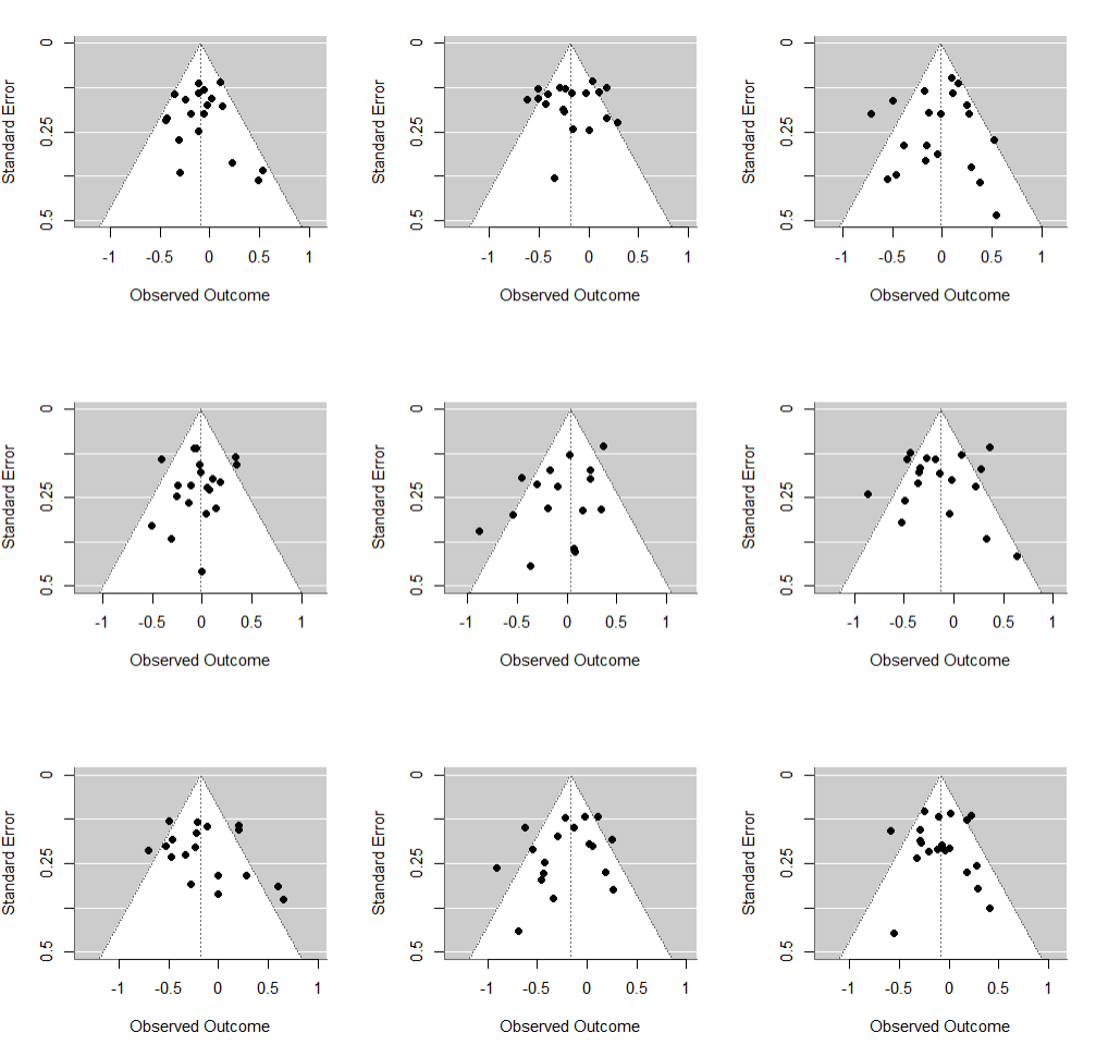
You can see that on average a few studies will fall outside of the funnel (rather than one, i.e. 5%). Why? Because the funnel is centered at the assumed true, fixed effect. It makes no provisions for effects in studies varying for reasons other than sampling variation.

However, now consider a situation where heterogeneity is driven by presence of distinct subgroups. We have 20 studies with true effect of -0.1 (same as above) and now add 5 more studies with much larger effect, -0.9. If we combine them in a single meta-analysis, the mean estimate will be somewhere around -0.25 (maths!), but funnel plots will look considerably more asymmetrical:

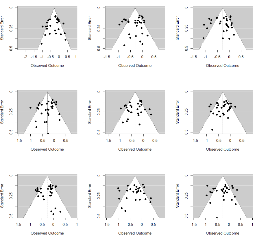
This type of asymmetry disappears once we conduct a subgroup analysis or regress on the covariate. The obvious challenge is that we often do not know about these systematic heterogeneity drivers, even if they are there: we just see a soup of disparate (and possibly a bit asymmetrical) estimates, very much like in the plot above.

Checking funnels: Egger’s test

The most typically used test Egger’s regression test: simply regress z-scores on reciprocal of standard errors.

• If the intercept is significantly different from zero, that suggests asymmetry
• You can modify the test in many ways (linear model vs meta-regression model, regressig on SEs vs variances vs N’s) and if you’re conducting the test in R, meta and metafor have different implementations.
• See R code at the end for a very simple demonstration.
• A simple modification for working with binary data was proposed by Peters et al, which avoids some false positives.

How to adjust for publication bias: Andrews and Kasy

Assume you suspect there is publication bias in your analysed sample of studies. We should be able not simply to test for it, but derive some kind of rule on how to penalise for it. A nice paper by Andrews and Kasy (2019) covers how to make this type of adjustment. The core idea is simple enough that it can be outlined in one paragraph and it should make intuitive sense to you.

Assume some heterogeneity, i.e. that the true effects in each study come from a normal distribution

\[\theta_k \sim \mathcal{N}(\mu, \tau^2)\]

(you can swap this for a Student’s T or another distribution, but a Gaussian is a typical choice). Each study now measures $\theta_k$ as a pair of mean effect and standard error:

\[\hat{\theta_k} \sim \mathcal{N}(\theta_k, se_k).\]

This is a standard random-effects model that can be estimated e.g. in baggr or any frequentist meta-analytic software. Now assume that researchers in study $k$ make publication decisions based on one quantity only, the signal to noise ratio $z_k = \hat{\theta_k} / se_k$. That is, we define some arbitrary function that assigns $z$ a publication probability $p(z)$.

\[\textrm{published}_k \sim \textrm{Bernoulli}(p(z_k))\]

We now have access only to studies where $\textrm{published}_k = 1$. However, Andrews and Kasy show that under these simple assumptions, if we assume we know the shape of $p(z)$, we can estimate it up to some constant. In plain language, if, for example, we assume something like a jump in publication likelihood when we meet the 5% significance threshold

\[p(z) = \begin{cases} c,\, \textrm{ if } \|z\| < 1.96, \\ c \delta \, \textrm{ otherwise},\\ \end{cases}\]

we can then estimate $\delta$, the relative publication probability. When we do that, we also retrieve the original parameters.

That means the Andrews and Kasy model returns the publication-bias adjusted quantities that the meta-analyst would be interested in. Of course for the method to work well in practice we need to have sufficient data on studies with $|z| < 1.96$ and $|z| \ge 1.96$ to carry out estimation.³

If this is still convoluted, you can think of the procedure graphically. For a basic $p(z)$ (symmetrical, with discontinuity at 5% significance level, i.e. 1.96) like above, we can think back to the funnel I drew earlier. (Let’s forget about heterogeneity for a moment and think of a fixed effect, just because it’s simpler that way.) Imagine you have lots of studies and start counting how many are inside and outside of the funnel. If you’ve got the right model and the process is simply governed by sampling variation, then you know 1 in 20 points should fall outside. Now, what if you have 900 studies inside the funnel and 100 outside? Well, it means you’re missing 1,000 in the middle. (See Figures 3 and 4 in the Andrews and Kasy paper for an illustration.) So under these assumptions you quickly get an idea of how much bias there is.

A frequentist implementation of this inference on $(\mu, \tau, \delta)$ is implemented not just in R and MATLAB, but also in a Shiny app by Kasy. See it here. (I just made up the notation above, mind.)

References

• Andrews, Isaiah, and Maximilian Kasy. ‘Identification of and Correction for Publication Bias’. American Economic Review 109, no. 8 (1 August 2019): 2766–94. https://doi.org/10.1257/aer.20180310.
• Peters, Jaime L., Alex J. Sutton, David R. Jones, Keith R. Abrams, and Lesley Rushton. ‘Comparison of Two Methods to Detect Publication Bias in Meta-Analysis’. JAMA 295, no. 6 (8 February 2006): 676–80. https://doi.org/10.1001/jama.295.6.676.
• Sterne, Jonathan A. C., Alex J. Sutton, John P. A. Ioannidis, Norma Terrin, David R. Jones, Joseph Lau, James Carpenter, et al. ‘Recommendations for Examining and Interpreting Funnel Plot Asymmetry in Meta-Analyses of Randomised Controlled Trials’. BMJ 343 (22 July 2011): d4002. https://doi.org/10.1136/bmj.d4002.

Appendix: R code for these demonstrations

# baggrdev/funnel_heterogen.R

library(metafor)
library(tidyverse)

# unexplained heterogeneity -----
b1 <- replicate(9, {
  rr  <- 0.9
  tau <- 0.2 #on log scale
  Ns <- 20
  true_rr <- exp(rnorm(Ns, log(rr), tau))
  N  <- runif(Ns, 100, 5000)
  p1 <- runif(Ns, 0.01, 0.10)
  n1 <- n2 <- round(N/2)
  c  <- rbinom(Ns, n2, p1)
  a  <- rbinom(Ns, n1, p1*true_rr)
  se <- sqrt(1/a + 1/c + 1/n1 + 1/n2)
  rr_hat <- log((a/n1)/(c/n2))
  df1 <- data.frame(a, c, n1, n2, se, rr_hat) %>% 
    dplyr::filter(!is.infinite(se))
}, simplify = F)

par(mfrow = c(3,3))

lapply(b1, function(x) {
  mf <- rma(data=x, yi=rr_hat, sei=se, method = "FE")
  funnel(mf, ylim = c(0,0.5))
})



# covariate driving heterogeneity -----

# block one
b1 <- replicate(9, {
  rr <- 0.9
  Ns <- 20
  N  <- runif(Ns, 100, 5000)
  p1 <- runif(Ns, 0.01, 0.10)
  n1 <- n2 <- round(N/2)
  c  <- rbinom(Ns, n2, p1)
  a  <- rbinom(Ns, n1, p1*rr)
  se <- sqrt(1/a + 1/c + 1/n1 + 1/n2)
  rr_hat <- log((a/n1)/(c/n2))
  df1 <- data.frame(a, c, n1, n2, se, rr_hat) %>% 
    dplyr::filter(!is.infinite(se))
}, simplify = F)

par(mfrow = c(3,3))

lapply(b1, function(x) {
  mf <- rma(data=x, yi=rr_hat, sei=se)
  funnel(mf, ylim = c(0,0.5))
})

# block two
b2 <- replicate(9, {
  rr <- 0.4
  Ns <- 5
  N  <- runif(Ns, 100, 5000)
  p1 <- runif(Ns, 0.01, 0.10)
  n1 <- n2 <- round(N/2)
  c  <- rbinom(Ns, n2, p1)
  a  <- rbinom(Ns, n1, p1*rr)
  se <- sqrt(1/a + 1/c + 1/n1 + 1/n2)
  rr_hat <- log((a/n1)/(c/n2))
  df2 <- data.frame(a, c, n1, n2, se, rr_hat) %>% filter(!is.infinite(se))
}, simplify = FALSE)

for(i in 1:9) {
  df <- rbind(b1[[i]], b2[[i]])
  mf <- rma(data=df, yi=rr_hat, sei=se)
  # print(ranktest(mf))
  print(regtest(mf))
  funnel(mf, ylim = c(0,0.5))
}


# publication bias -----
pr_signif <- 1
pr_nonsignif <- 0.25

bpb <- replicate(9, {
  rr  <- 0.9
  tau <- 0.2 #on log scale
  Ns <- 50
  true_rr <- exp(rnorm(Ns, log(rr), tau))
  N  <- runif(Ns, 100, 5000)
  p1 <- runif(Ns, 0.01, 0.10)
  n1 <- n2 <- round(N/2)
  c  <- rbinom(Ns, n2, p1)
  a  <- rbinom(Ns, n1, p1*true_rr)
  se <- sqrt(1/a + 1/c + 1/n1 + 1/n2)
  rr_hat <- log((a/n1)/(c/n2))
  
  df1 <- data.frame(a, c, n1, n2, se, rr_hat) %>% 
    dplyr::filter(!is.infinite(se)) %>% 
    mutate(signif = 1*(abs(rr_hat) - 1.96*se > 0)) %>% 
    mutate(pub_pr = ifelse(signif, pr_signif, pr_nonsignif)) %>% 
    mutate(publication = rbinom(nrow(.), 1, pub_pr)) %>% 
    filter(publication == 1)
  
}, simplify = F)

par(mfrow = c(3,3))

# This is how Egger's regression test works
library(meta)
mg <- metagen(TE = rr_hat, seTE = se, data = bpb[[9]])
metabias(mg, method.bias = "linreg")

# you could just do that by hand:
mutate(bpb[[9]],y = rr_hat/se, x = 1/se) %>% 
  lm(data = ., y ~ x) %>% summary 

# but in metafor this is done differently under default settings
# and there is a choice of different predictors
mf <- rma(data=bpb[[9]], yi=rr_hat, sei=se, method = "FE")
regtest(mf, predictor = "se", model = "lm")
regtest(mf) #but the default model is `rma`

1. Thinking of results as simply published or not can be reductive. You can also think of results that were published somewhere, but cannot be accessed because they had no exposure or haven’t been indexed in search, they are no longer available, not yet available, they are in a different language etc. So in a broader sense “published” means “I can find what I need when looking for data to analyse”. Consider that studies may have been conducted but then selective in terms of what they reported: for example, in a meta-analysis of water treatment we found that researchers didn’t report on child mortality, because it was so rare (very typically single digit numbers of deaths may occur), even though they had these data. ↩

2. Also note an interesting association between intervention effect and standard error that occurs by design. Early studies of an intervention are typically small. As we learn more about the intervention, we both start calibrating the sample sizes, because we get a better sense of what the effect size may be that we’re trying to detect. We also evolve study protocols and intervention designs, which may lead to different effect sizes in subsequent studies. So in some domains there will be a relationship between sample sizes and effects. (For this point I am indebted to Michael Kremer.) ↩

3. There is an extra complication, which I alluded to in an earlier footnote. The inference assumes that standard errors and effect sizes are independent. But we know that this is unlikely to be the case in many domains. I don’t have a good intuition on how much of a problem that presents. Unfortunately, it seems like all publication bias assessment methods just assume that. ↩